How to Calculate Static Pressure in an HVAC System
Calculate static pressure at design stage, measure TESP at commissioning and compare the two to diagnose excess resistance.
Static pressure is the pressure air exerts against the walls of a duct. In an HVAC system, changes in static pressure show how much resistance the airflow encounters as it moves through ducts, filters, coils, fittings and terminals.
Get it wrong at design stage and the blower can’t deliver design airflow, so coils lose capacity and rooms miss their loads. It’s also a number you can check after installation, which makes it a fast test of whether what was built matches what you drew.
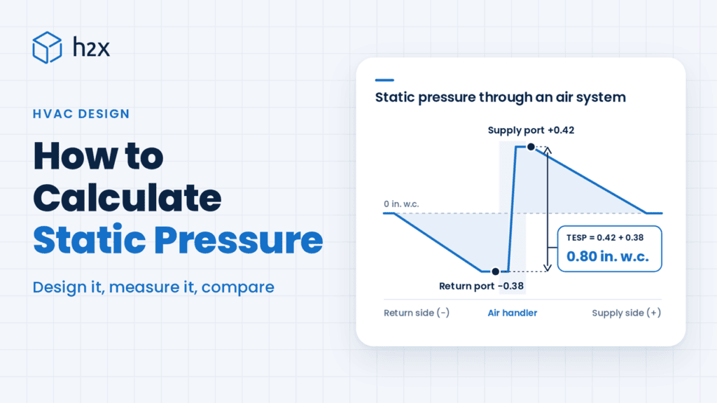
You measure it in the field as total external static pressure (TESP), adding the supply and return readings as absolute values. You calculate it at design stage as the friction loss along the index run plus fitting and component losses, using Darcy-Weisbach for the friction term.
Technicians measure and engineers calculate, and the two rarely meet on one job. This guide does both on one illustrative system: a 2,400 ft² (223 m²) Atlanta house, sized to a calculated friction rate, then checked with a manometer. The commercial case follows for readers in the UK and Australia and New Zealand (ANZ), where the discipline is usually called mechanical or building services rather than HVAC.
Quick Answer: To calculate static pressure in an HVAC system, measure it in the field as total external static pressure (TESP): add the supply and return readings as absolute values. At design stage, subtract component losses from the blower’s rated TESP, then spread the rest across the index run’s total effective length to get the friction rate.
Key Takeaways
- Field method: Total external static pressure is the supply reading plus the return reading, added as absolute values, because the return side reads negative.
- Design method: Subtract component losses from the blower’s rated TESP, then spread the rest across the index run’s total effective length. That gives the friction rate you size ducts to.
- Velocity pressure: Total pressure is static plus velocity pressure. You can’t read velocity pressure directly: a pitot tube gives total and static pressure, and velocity pressure is the difference.
- Diagnostic threshold: A TESP more than 10% to 20% above the maximum rated value probably means an airflow problem, according to Rob Falke of the National Comfort Institute (NCI), writing on the Air Conditioning Contractors of America (ACCA) blog.
- Units: One inch of water column (in. w.c.) equals 249.09 pascals (Pa), so a 0.50 in. w.c. rating is 124.5 Pa and a 0.70 in. w.c. rating is 174 Pa.
- Fan laws: On a fixed system, pressure rises with the square of fan speed and power with the cube. Speeding up a blower to beat a restriction costs far more power than it recovers in airflow.
Why Static Pressure Matters, and When to Calculate or Measure It
Static pressure is what the system’s resistance consumes. Every foot of duct, every elbow, the filter, coil, grille and damper takes a slice, and the fan must deliver their sum at the design airflow.
Move less air than assumed over a cooling coil and you get colder supply air, lost capacity and a risk of coil icing. That’s why static pressure matters more than almost any other number a duct designer picks.
It’s also the number that decides whether the rest of the design is deliverable. An airflow you can’t push through the ductwork at the pressure the blower has isn’t a design, and the failure shows up at commissioning rather than on the drawing.
The two methods answer different questions and you need them at different moments.
| When you’re | What you do | What it tells you |
|---|---|---|
| Designing, before anything is installed | Calculate: component losses off rated TESP, the remainder spread across the index run | What the system should need, and therefore what duct sizes to draw |
| Selecting a fan | Calculate along the index run, on total pressure for commercial work | The duty to buy against |
| Commissioning a new system | Measure TESP and compare it with the design figure | Whether what was built matches what was drawn |
| Diagnosing a complaint on an existing system | Measure first, split supply against return, then calculate what it should have been | Where the extra resistance is |
| Retrofitting equipment into existing ducts | Both: measure the existing system, then recalculate the friction rate on the new blower’s rated TESP | Whether the existing ducts can carry the new airflow |
The design number without a field check is an assumption. The field reading without a design number is a reading with no reference. The worked example below does both on one system for exactly that reason.
What Are Static, Velocity and Total Pressure?
Total pressure is static pressure plus velocity pressure, in both US and Chartered Institution of Building Services Engineers (CIBSE) terminology. Static pressure acts outward on the duct wall whichever way the air travels. Velocity pressure belongs to the air’s motion and acts only along the flow.
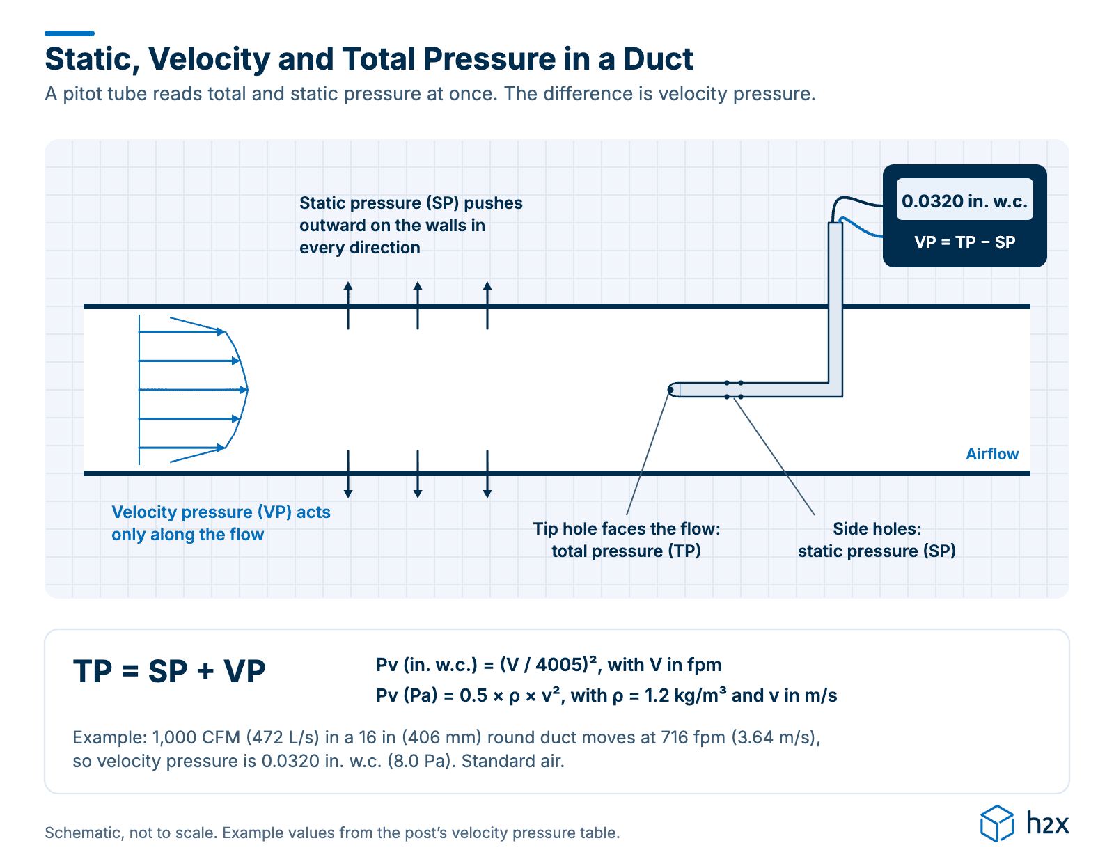
You can’t read velocity pressure off a gauge alone. Measure total and static pressure with a pitot tube and a differential pressure sensor, and take the difference.
TP = SP + VP

Pv = (V / 4005)²        imperial, in. w.c.

Pv = 0.5 × ρ × v²       SI, Pa
- TP = total pressure; SP = static pressure; VP or Pv = velocity pressure
- V = air velocity in feet per minute (fpm)
- v = air velocity in m/s
- ρ = air density, 1.2 kg/m³ for standard air
The 4005 constant comes from gravity, water density, inches per foot, standard air at 0.075 lb/ft³ (1.2 kg/m³), and 60 to convert ft/s to fpm:
4005 = 60 × √((2 × 32.1722 × 62.3215) / (12 × 0.075))
It holds only for standard air. For other densities, use:
V = 1097 × √(Pv / d)
- d = air density in lb/ft³
The table holds airflow at 1,000 cubic feet per minute (CFM), or 472 L/s, through four diameters, so only velocity changes.
| Duct, in (mm) | Area, ft² (m²) | Velocity, fpm (m/s) | Pv (in. w.c.) | Pv (Pa) | SI check, 0.5 × 1.2 × v² (Pa) |
|---|---|---|---|---|---|
| 16 (406) round | 1.3963 (0.1297) | 716 (3.64) | 0.0320 | 8.0 | 7.9 |
| 14 (356) round | 1.0690 (0.0993) | 935 (4.75) | 0.0546 | 13.6 | 13.5 |
| 12 (305) round | 0.7854 (0.0730) | 1,273 (6.47) | 0.1011 | 25.2 | 25.1 |
| 10 (254) round | 0.5454 (0.0507) | 1,833 (9.31) | 0.2096 | 52.2 | 52.1 |
Standard air at 0.075 lb/ft³ (1.2 kg/m³). Imperial and SI agree within 0.1 Pa, which is rounding in the constants. Project data governs.
Squeezing that trunk from 16 in (406 mm) to 10 in (254 mm) multiplies velocity pressure by 6.6, because the velocity term is squared. That squared term is why an undersized duct shows up so fast as high static pressure, and why it pays to know how to find air velocity in a duct.
The National Institute of Standards and Technology (NIST) lists an inch of water column in Special Publication 811. It’s 249.082 Pa at 39.2 °F (4 °C) and 248.84 Pa at 60 °F (15.6 °C), a difference of about 0.1%. We use NIST’s conventional value, 249.09 Pa.
How Do You Calculate Static Pressure at Design Stage?
At design stage there’s no manometer, so you compute the loss with the Darcy-Weisbach equation. It applies to air and water alike, which is why water-side shortcuts such as Hazen-Williams are judged against it.
Δp = f × (L / Dh) × (ρ × v² / 2)                 pressure form, Pa

Δh = f × (L / Dh) × (ρf / ρwater) × (v² / 2g)    head form
- Δp = pressure loss (Pa); Δh = head loss, as a height of water column
- f = Darcy friction factor (dimensionless)
- L = duct length (m); Dh = hydraulic diameter (m)
- ρ = air density (kg/m³); ρf = fluid density; ρwater = water density
- v = mean air velocity (m/s); g = gravitational acceleration (m/s²)
The Friction Factor
The friction factor depends on flow regime and duct roughness, and the Reynolds number sets the regime.
Re = ρ × v × D / μ = v × D / ν

Laminar, Re below 2,000:     f = 64 / Re

Colebrook-White:             1 / √f = -2 × log10[(ε / D) / 3.7 + 2.51 / (Re × √f)]

Swamee-Jain:                 f = 0.25 / [log10((ε / D) / 3.7 + 5.74 / Re^0.9)]²
- Re = Reynolds number (dimensionless)
- D = duct diameter (m); ε = absolute roughness of the duct wall (m)
- μ = dynamic viscosity (Pa·s); ν = kinematic viscosity (m²/s)
Colebrook-White is the turbulent reference correlation, but it has f on both sides and must be iterated. Swamee and Jain (1976) give an explicit form that stays within about 1% of it across its stated range. That’s why Swamee-Jain goes in a spreadsheet, and there’s more in our guide to the Darcy friction factor.
A duct friction chart or ductulator is that calculation pre-solved for standard air at 0.075 lb/ft³ (1.2 kg/m³) and galvanized steel with an absolute roughness of 0.0003 ft (0.09 mm), the “Average” roughness category in Table 1 of Chapter 21, Duct Design, in the 2017 ASHRAE Handbook, Fundamentals. You read a friction rate straight off CFM and diameter without iterating, but change either assumption and the chart is wrong. Our air duct pressure drop calculation guide goes further.
Fittings and Total Effective Length
Elbows, takeoffs, boots and transitions lose pressure through turbulence, not wall friction. So each is expressed as the straight-duct length that would lose the same pressure at the same airflow. Physical length plus fitting equivalent lengths gives total effective length (TEL).
In the example below, the supply side is 52 ft (15.8 m) of physical duct plus 168 ft (51.2 m) of fittings, so 220 ft (67 m). The return is 28 ft (8.5 m) plus 112 ft (34.1 m), so 140 ft (43 m). TEL is 220 + 140 = 360 ft (110 m), and the fittings carry more effective length than the ductwork, so you can’t skip the fitting count.
The friction rate follows:
FR = (ASP × 100) / TEL      imperial, in. w.c. per 100 ft

FR = ASP / TEL              SI, Pa/m
- FR = friction rate
- ASP = available static pressure: rated TESP minus component pressure losses (in. w.c. or Pa)
- TEL = total effective length of the index run (ft or m)
h2x design software recalculates duct sizes and pressure drop as you draw, so the friction rate and the duct sizes can’t drift apart.
How Much Static Pressure Do Filters, Coils and Grilles Take?
Components take their share before any pressure reaches the ductwork, so subtract them first. Filter ratings below use the minimum efficiency reporting value (MERV) scale.
| Component | Pressure loss (in. w.c.) | Pressure loss (Pa) | Source |
|---|---|---|---|
| Filter, 1 in. option, maximum specified drop at design airflow (California) | 0.10 | 25 | 2025 Title 24, Section 150.0(m)12B |
| Filter, ACCA worked example | 0.18 | 44.8 | Verifying ACCA Manual D Procedures |
| Direct expansion cooling coil, ACCA worked example | 0.23 | 57.3 | Verifying ACCA Manual D Procedures |
| Supply outlet, ACCA worked example | 0.03 | 7.5 | Verifying ACCA Manual D Procedures |
| Return grille, ACCA worked example | 0.03 | 7.5 | Verifying ACCA Manual D Procedures |
| Balancing damper, ACCA worked example | 0.03 | 7.5 | Verifying ACCA Manual D Procedures |
| MERV 13 filter, 1 in. (25 mm) deep, at 350 fpm (1.78 m/s), initial resistance | 0.49 | 122 | Camfil AP-Thirteen SC product sheet |
| MERV 13 filter, 4 in. (102 mm) deep, at 500 fpm (2.54 m/s), initial resistance | 0.37 | 92.2 | Camfil AP-Thirteen SC product sheet |
Reference points, not design values. Manufacturer and project data govern.
The Camfil figures are the maximum initial resistance of a clean filter at its rated face velocity. A loaded filter runs higher: Camfil recommends a maximum final resistance of 1.0 in. w.c. (249 Pa).
A high-MERV filter isn’t the problem on its own: depth and face area are. Camfil rates its 4 in. MERV 13 at 0.37 in. w.c. (92.2 Pa) at 500 fpm (2.54 m/s). That’s lower than its 1 in. MERV 13 at 0.49 in. w.c. (122 Pa), even though the thinner filter is rated at a slower 350 fpm (1.78 m/s).
California’s 2025 Energy Code (Title 24) gives several ways to comply. If you use a 1 in. filter, the filter or grille must be sized for a face velocity of 150 fpm (0.76 m/s) or less, and the filter must be specified with a drop of 0.1 in. w.c. (25 Pa) or less at the return’s design airflow. Outside California that’s a useful benchmark, not a requirement.
A wet coil loses more than a dry coil at the same face velocity, because condensate obstructs the air path. We didn’t find a published numeric difference, so use the manufacturer’s wet-coil figure. On dampers, Greenheck’s control damper catalog specifies opposed-blade dampers for modulating airflow and parallel-blade dampers for two-position duty.
How Do You Measure Total External Static Pressure?
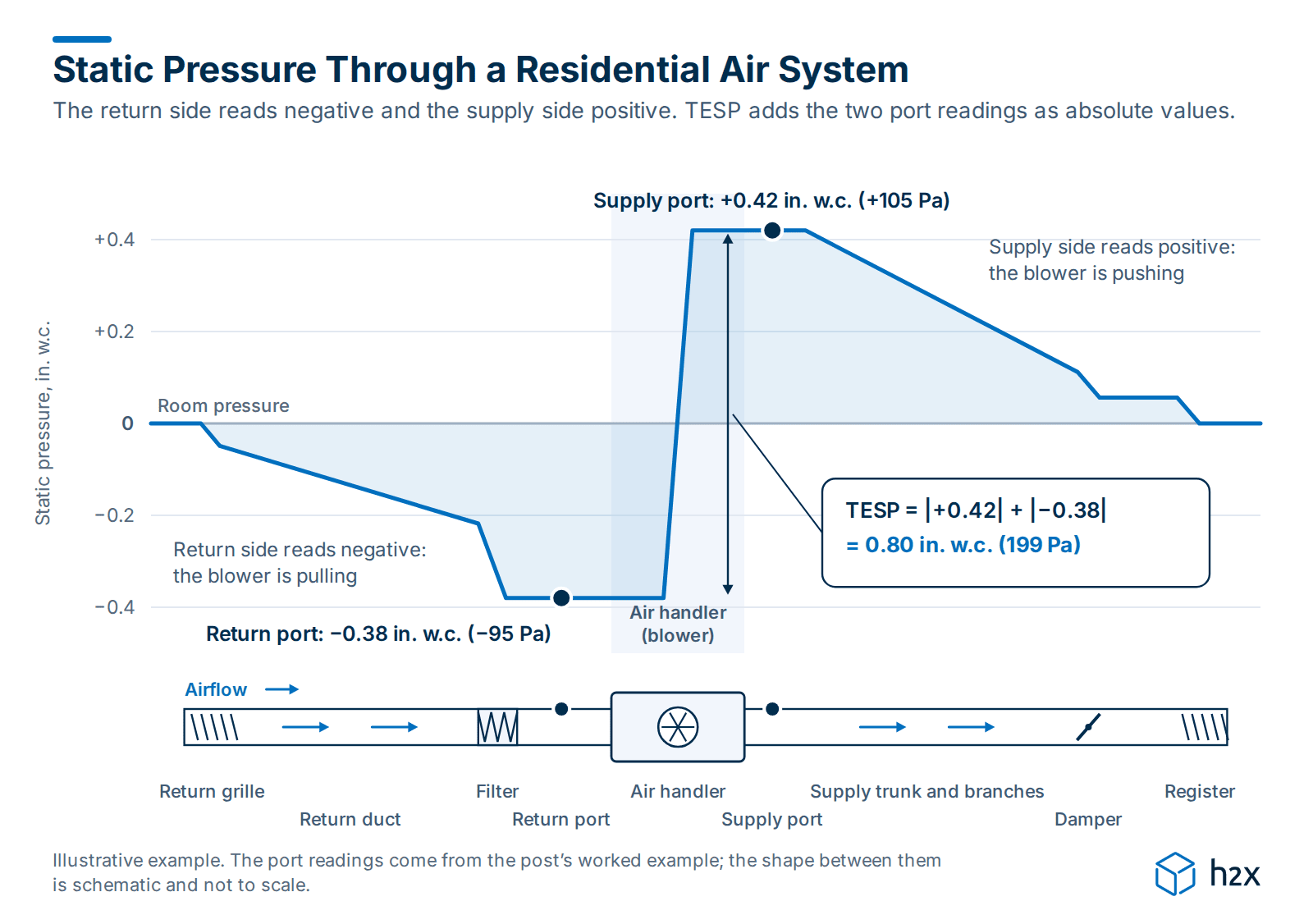
Two ports, two readings, one sum.
- Return side: between the filter and the blower inlet. It reads negative, because the blower is pulling.
- Supply side: where air leaves the equipment, after an air handler’s cabinet or between a furnace and its add-on coil. It reads positive.
TESP = |supply reading| + |return reading|
- TESP = total external static pressure (in. w.c. or Pa)
Sum the absolute values, because the ports sit either side of the fan.
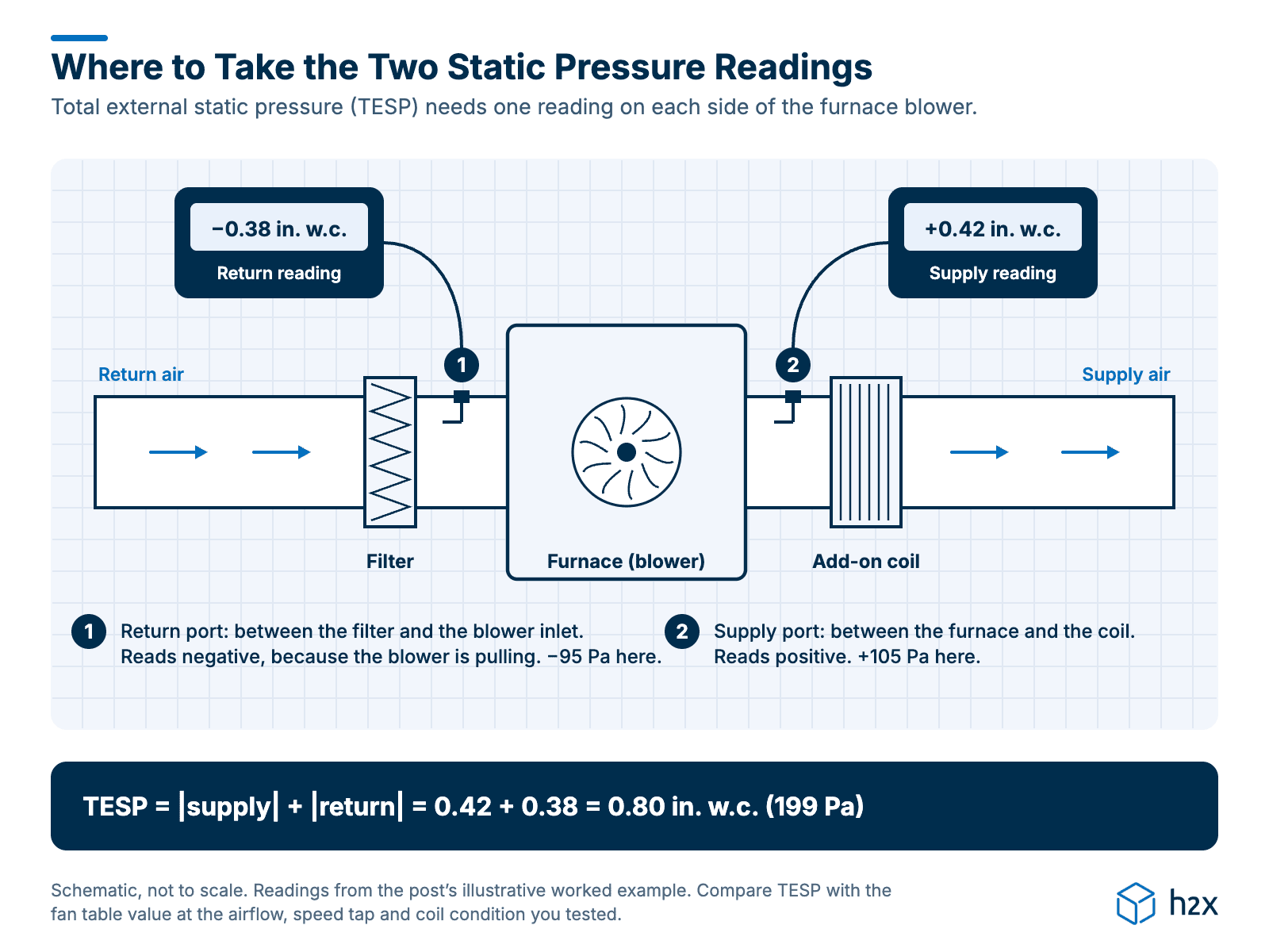
Three things must match before the reading means anything:
- Coil condition: fan tables give separate TESP-versus-CFM curves for cooling with a wet coil and for heating-only operation, so read the curve for the mode you’re testing in.
- Speed tap: fan tables are stated per tap.
- Reference value: use the fan table figure at the actual airflow, not the nameplate headline.
Rated TESP is the pressure the blower is engineered to overcome outside its own cabinet, at a stated airflow and speed tap. The US Department of Energy (DOE) furnace fan test procedure sets 0.50 to 0.55 in. w.c. (124.5 to 137 Pa) for units with a factory-installed coil, and 0.65 to 0.70 in. w.c. (162 to 174 Pa) for units designed to be paired with a separate coil. That’s in 10 CFR 430, Subpart B, Appendix AA, Table 1.
For electronically commutated motor (ECM) equipment, ACCA’s Manual D has told designers since its 2014 revision to use 0.70 in. w.c. (174 Pa) as the maximum design external static pressure. ACCA’s Luis Escobar explains the change. Either way, read the actual fan table.
Worked Example of Design Intent Versus Field Reading on One System
Take a 2,400 ft² (223 m²) house in Atlanta, Georgia, with a design airflow of 1,000 CFM (472 L/s), about 2.5 tons of cooling at 400 CFM per ton, and its ducts inside the conditioned envelope. It has a variable-speed furnace with an add-on cased evaporator coil, and the furnace blower is rated at 0.70 in. w.c. (174 Pa) TESP at that airflow.
Step 1. What the Design Said
| Component | Pressure loss (in. w.c.) | Pressure loss (Pa) |
|---|---|---|
| Filter, 4 in. MERV 13, clean, 20 × 25 in face (288 fpm, 1.46 m/s face velocity) | 0.15 | 37.4 |
| Add-on evaporator coil, wet | 0.24 | 59.8 |
| Supply registers | 0.03 | 7.5 |
| Return grille | 0.03 | 7.5 |
| Balancing dampers | 0.03 | 7.5 |
| Total component pressure losses (CPL) | 0.48 | 119.6 |
Design allowances for this equipment selection. Manufacturer and project data govern. The filter allowance is read from Camfil’s resistance curve for a clean filter at 288 fpm (1.46 m/s), well below its 500 fpm (2.54 m/s) rating point, which is why it’s lower than the 0.37 in. w.c. (92.2 Pa) in the component table.
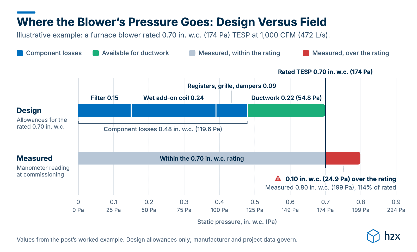
ASP = TESP - CPL = 0.70 - 0.48 = 0.22 in. w.c. (54.8 Pa)

TEL = 220 + 140 = 360 ft (110 m)

FR = (ASP × 100) / TEL = (0.22 × 100) / 360 = 0.061 in. w.c. per 100 ft

FR (SI) = 54.8 / 110 = 0.50 Pa/m
- ASP = available static pressure; TESP = the furnace blower’s rated TESP
- CPL = total component pressure losses from the table
- TEL = total effective length; FR = friction rate
The coil counts as a component loss here because it sits outside the furnace cabinet. An air handler is different: its coil is inside the cabinet, and the fan table already includes the dry-coil loss.
The Bryant FV4C fan coil data, for example, is rated with a dry coil and filter in place, with a separate dry-to-wet correction of 0.022 in. w.c. (5.5 Pa) at 800 CFM (378 L/s) on its smallest size. With an air handler, subtract only that wet-coil correction and anything the rating excludes. Never subtract the whole coil a second time.
At that rate the trunk calculates to 15.10 in (384 mm) and is built as 16 in (406 mm) round, carrying 1,000 CFM (472 L/s) at 716 fpm (3.64 m/s). Defaulting to 0.10 in. w.c. per 100 ft (0.82 Pa/m) would have sized every duct for 1.64 times the pressure available.
Step 2. What the Manometer Said
Say the technician runs the system in cooling, on the tap the fan table was read at, and gets these readings:
- Supply, between furnace and coil: +0.42 in. w.c. (+105 Pa)
- Return, between filter and blower: -0.38 in. w.c. (-95 Pa)
TESP = |0.42| + |-0.38| = 0.80 in. w.c. (199 Pa)
Step 3. The Diagnostic Ratio
The measured 0.80 in. w.c. against a rated 0.70 in. w.c. is 114% of rated, or 14% over. Rob Falke, president of the National Comfort Institute, writes on the ACCA blog that a TESP more than 10% to 20% above maximum rated TESP probably means an airflow problem degrading performance.
Step 4. Where the Extra 0.10 in. w.c. Went
The gap is 0.80 minus 0.70, or 0.10 in. w.c. (24.9 Pa). There are four usual suspects: a loaded filter, an undersized return, a compressed flexible duct run or a closed damper.
The two readings show which side it’s on. The filter and return grille sit on the return side of the blower, and the coil, registers and dampers on the supply side, so the design split the 0.70 in. w.c. (174 Pa) like this:
Return, design = 0.15 + 0.03 + (140 × 0.061 / 100) = 0.27 in. w.c. (67 Pa)

Supply, design = 0.24 + 0.03 + 0.03 + (220 × 0.061 / 100) = 0.43 in. w.c. (107 Pa)
The supply reads +0.42 in. w.c. (+105 Pa), right on design. The return reads -0.38 in. w.c. (-95 Pa), 0.11 in. w.c. (27 Pa) over. The extra resistance is on the return side, which points away from the supply dampers.
Start with the filter, because it’s the cheapest check. Measure on both sides of it, and the difference is what it’s actually costing against the 0.15 in. w.c. (37.4 Pa) the design allowed.
If the filter is within its allowance, look at the return duct. The return trunk carries the same 1,000 CFM (472 L/s) as the supply trunk, and compressed flex has the largest multiplier, at the same 0.061 in. w.c. per 100 ft (0.50 Pa/m):
| Duct | Friction multiplier | Required diameter, in (mm) | Use, in (mm) |
|---|---|---|---|
| Rigid galvanized metal | 1.0× | 15.10 (384) | 16 (406) |
| Flex at about 15% compression (ADC) | 2.0× | 17.40 (442) | 18 (457) |
| Flex at about 30% compression (ADC) | 4.0× | 20.06 (509) | 22 (559) |
| Flex, heavily compressed (lab tests) | about 10× | 24.23 (615) | 26 (660) |
The 2× and 4× multipliers are from the Air Diffusion Council (ADC) Flexible Duct Performance & Installation Standards, 5th edition. Lawrence Berkeley National Laboratory (LBNL) found that further compression raised pressure drop by factors close to ten. Texas A&M tests found some compressed configurations lost over ten times as much pressure as rigid or fully stretched duct of the same diameter (Weaver and Culp, 2006). Project data governs.
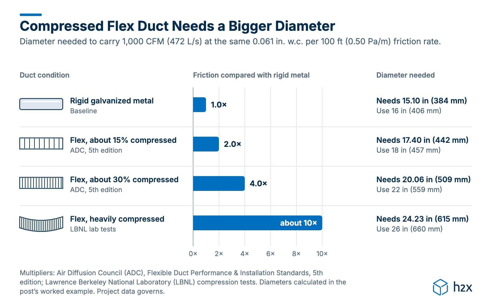
A 16 in (406 mm) return trunk in flex at 15% compression needs 17.40 in (442 mm) to hold the design friction rate. It should have gone in as 18 in (457 mm). Built at 16 in, it runs at about 0.092 in. w.c. per 100 ft (0.75 Pa/m), 1.5 times the friction rate the rest of the system assumes.
Step 5. Why a Variable-Speed Blower Hides the Problem
A permanent split capacitor (PSC) blower loses airflow as static pressure rises, along its fan table. An ECM blower ramps motor speed to hold airflow instead, at the cost of higher power draw, motor stress and noise. That means a variable-speed blower hides a duct problem instead of announcing it, so take the reading anyway.
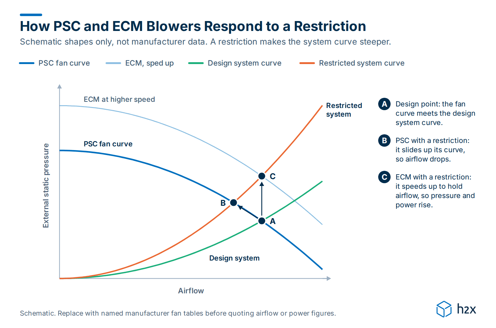
Goodman’s published fan tables show the difference on two 60,000 BTU/h furnaces, each rated for up to 3 tons of cooling airflow. The GMS80603, with a multi-speed PSC motor on its high tap, drops from 1,157 CFM at 0.50 in. w.c. to 1,075 CFM at 0.70 in. w.c. (546 to 507 L/s at 124.5 to 174 Pa). That’s 7% less air.
The variable-speed GMVC960603 on cooling tap D holds 1,212 CFM (572 L/s) anywhere from 0.1 to 0.8 in. w.c. (25 to 199 Pa). One table tells you the ducts are restrictive. The other won’t.
Why a Small Pressure Problem Becomes a Large Power Problem
For a fixed system at varying fan speed, the fan laws are:
Q2 / Q1 = n2 / n1

Δp2 / Δp1 = (n2 / n1)²

P2 / P1 = (n2 / n1)³
- Q = airflow; n = fan speed; Δp = fan pressure; P = fan power
- 1 and 2 = the conditions before and after the speed change
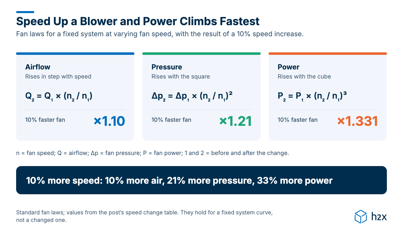
| Speed change | Airflow | Pressure | Power |
|---|---|---|---|
| ×1.10 | ×1.10 | ×1.21 | ×1.331 |
| ×0.90 | ×0.90 | ×0.81 | ×0.729 |
| ×0.80 | ×0.80 | ×0.64 | ×0.512 |
A 10% speed increase buys 10% more air for 21% more pressure and 33% more power. So if you recover lost airflow by speeding up the blower instead of fixing the restriction, every 10% of airflow costs about a third more power.
How Do You Correct Static Pressure for Altitude?
Air density is proportional to barometric pressure divided by absolute temperature. Gain altitude and barometric pressure falls; heat the air and absolute temperature rises. Either way density falls.
Because density sits in the ρ × v² / 2 term, the pressure drop at a given airflow is lower than standard-air charts predict.
| Site elevation, ft (m) | Air density correction factor |
|---|---|
| Below 3,000 (914) | 1.000 |
| 3,000 to under 4,000 (914 to under 1,219) | 0.896 |
| 4,000 to under 5,000 (1,219 to under 1,524) | 0.864 |
| 5,000 to under 6,000 (1,524 to under 1,829) | 0.832 |
| 6,000 (1,829) and above | 0.801 |
From Table 140.4-C of the 2025 California Energy Code (Title 24, Part 6), a fan-power compliance table. The table number and values are unchanged from the 2022 code. Cite it as such: it isn’t a universal HVAC altitude reference, and it assumes standard air temperature.
Temperature matters as much as altitude. The chart below corrects for both, using the US Standard Atmosphere and the ideal gas law, and its 70 °F (21 °C) row matches the Title 24 factors within 0.01.
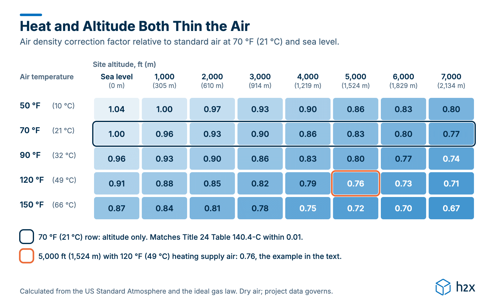
For contrast, move the worked example’s system from Atlanta to a site at 5,000 ft (1,524 m), close to Denver’s elevation. At 70 °F (21 °C) the correction factor is 0.83, so the 16 in (406 mm) trunk’s velocity pressure falls from 0.0320 to about 0.027 in. w.c. (8.0 to 6.6 Pa) at the same 1,000 CFM (472 L/s). In heating, with 120 °F (49 °C) supply air, the factor at that altitude drops to 0.76.
The lower pressure drop is only half the picture. If you raise airflow to move the same mass of air as at sea level, two corrections apply and they push opposite ways. Lower density reduces pressure at a fixed airflow, but pressure rises with the square of airflow, and that’s the larger term. Net at 5,000 ft (1,524 m):
- Airflow: 1 / 0.83 = 1.20, so 20% more CFM for the same mass flow
- Pressure: 0.83 × (1 / 0.83)² = 1.20, so 20% more static pressure than the same duty at sea level
- Power: 0.83 × (1 / 0.83)³ = 1.45, so about 45% more fan power
That’s the counterintuitive part: the blower needs more power at elevation, not less. Take elevation and supply air temperature into account at design stage, correct the fan table for density and check the blower can deliver the corrected duty.
What Causes High or Low Static Pressure?
High static pressure means resistance exceeds the design assumption. The usual causes are undersized ducts, undersized or restricted returns, compressed or kinked flex, a loaded filter or a throttled damper. A coil dirtier or wetter than assumed does the same, and so do too many fittings on the index run.
Airflow then drops, and in cooling the lower airflow over the coil drops coil temperature, cutting capacity and raising the risk of coil icing. In heating, supply temperature climbs toward the high limit. In both modes a variable-speed blower draws more power, and duct noise rises with velocity.
| Measured TESP vs fan table value | Likely meaning | First checks |
|---|---|---|
| At or below rated | Inside the design envelope | Airflow, coil condition |
| Up to 10% over | Minor accumulated resistance | Filter, damper positions |
| 10-20% over | Investigate band (Falke, NCI) | Split supply against return |
| More than 20% over | A real restriction | Return sizing, flex, coil, index run |
| Well below expectation | Pressure bypassing what you measure | Disconnected duct, missing filter, wrong tap |
The 10% to 20% band comes from Rob Falke of the National Comfort Institute, writing on the ACCA blog. The other rows follow from the pressure balance rather than a published threshold, and low static pressure is far less documented than high.
Attribute prevalence carefully. A 2002 LBNL paper for the American Council for an Energy-Efficient Economy (ACEEE) cites Proctor and Parker (2000). Across nine field studies with a combined sample of 245 systems, Proctor and Parker measured external static pressures two to four times higher than the DOE test assumptions of the time.
Those assumptions were 0.1 to 0.2 in. w.c. (25 to 50 Pa), against field values of 0.41 to 0.55 in. w.c. (102 to 137 Pa) in the air conditioning studies. We haven’t found a large-sample peer-reviewed prevalence figure more recent than that.
How Is Static Pressure Handled in Commercial Systems?
Commercial practice in the UK and ANZ shifts the emphasis to total pressure. A CIBSE Journal CPD module notes that working in total pressure is useful for clarity when selecting fans. The velocity pressure leaving the fan outlet is energy the fan must supply, so selecting on static pressure alone under-selects by that amount.
The path that sizes the fan is the index run, or index circuit: the path with the highest total pressure loss from fan to terminal. Every other path is balanced down to it, which is the same concept as Manual D’s most restrictive run, expressed in Pa rather than in. w.c.
In a low-velocity system, straight ductwork typically loses around 0.12 in. w.c. per 100 ft (1 Pa/m), according to the same continuing professional development (CPD) module. The same module works an example of circular steel duct at 0.16 in. w.c. per 100 ft (1.3 Pa/m), read from CIBSE Guide C (2007). Over 16.4 ft (5 m), that gives 0.026 in. w.c. (6.5 Pa).
In ANZ, training material from the Australian Institute of Refrigeration, Air Conditioning and Heating (AIRAH) reports a rule of thumb of sizing ducts at 0.15 in. w.c. per 100 ft (1.2 Pa/m), for airflows of about 380 to 9,500 CFM (180 to 4,500 L/s). It notes that’s higher than many designers use.
Clause J6D7 of the National Construction Code (NCC) 2025, Volume One covers ductwork in air-conditioning systems of about 6,400 CFM (3,000 L/s) or more. It requires that ductwork to be sealed to AS 4254.1:2021 (flexible duct) and AS 4254.2:2012 (rigid duct) for the system’s static pressure, unless it’s inside the only or last room the system serves. The clause is unchanged from NCC 2022, which some states still apply until 1 May 2027.
Common Mistakes When Measuring and Calculating Static Pressure
- Reading only the supply side. Take both readings and add them as absolute values, because the supply reading alone (0.42 in. w.c., or 105 Pa, above) hides a system that’s 14% over rated.
- Comparing against the wrong fan table value. Read the curve for the coil condition, speed tap and actual airflow you tested at, not the nameplate headline.
- Commissioning on a clean filter without noting it. Record the filter’s condition with the reading, because the filter only gets dirtier from there.
- Calculating along the shortest run instead of the index run. Size on the path with the highest total pressure loss, because the fan has to serve the worst path.
- Using a standard-air friction chart at altitude. Apply a density correction, such as Title 24’s factor of 0.801 at 6,000 ft (1,829 m) and above, before trusting the chart’s pressure drops.
- Selecting a commercial fan on static pressure alone. Select on total pressure, because the fan also has to supply the velocity pressure at its outlet.
How h2x Helps with Static Pressure Calculations
h2x is a cloud design platform for mechanical, plumbing and wet fire protection. You draw the ductwork over an imported PDF or DWG, and h2x sizes each section and calculates its pressure drop as you draw.
Move a diffuser or swap in a revised floor plan and it recalculates, so the friction rate, velocities and index run update together. Real-time error checking flags problems while you’re still drawing, not at commissioning.
The System Sizing Report lists size, airflow, velocity and pressure drop for every section and identifies the index run. That’s the audit trail a design reviewer wants. h2x’s heating and cooling water, domestic water and ventilation calculations are verified by CIBSE, and h2x’s calculations are aligned with ASHRAE methods.
h2x doesn’t design refrigerant pipework or full air conditioning systems, so pair it with a dedicated tool for that part.
Conclusion
Static pressure is one quantity with two methods, and the value is in comparing them. Calculate it at design stage by subtracting component losses from the blower’s rated TESP and spreading the rest across the index run’s total effective length. Then measure it at commissioning with two ports and a manometer, and investigate readings more than 10% to 20% above the maximum rated TESP for excess resistance.
Frequently Asked Questions
How do you calculate static pressure in an HVAC system?
In the field, add the supply and return readings as absolute values to get total external static pressure, because the return reads negative. At design stage, subtract component losses from the blower’s rated TESP. Then divide the remainder across the index run’s total effective length, with each section’s friction from Darcy-Weisbach.
What is a good static pressure reading?
A suitable reading is one that falls within the manufacturer’s blower data at the required airflow and operating condition. Rob Falke of the National Comfort Institute treats more than 10% to 20% over maximum rated TESP as an airflow problem. For ECM equipment, Manual D tells designers to use 0.70 in. w.c. (174 Pa) as the maximum design static pressure.
What is the difference between static pressure and total external static pressure?
Static pressure is the pressure air exerts in all directions, measured perpendicular to the flow at a single point. It’s the static part of total pressure = static pressure + velocity pressure, and it’s the part available to push air through resistance. It reads positive on the supply side and negative on the return.
Total external static pressure is a system-level number: the static resistance the blower must overcome outside its own cabinet, measured as supply static minus return static, which is the same as adding the two readings as absolute values. “Total” means both sides added together, not static plus velocity, so TESP contains no velocity pressure. “External” means losses inside the cabinet, such as an air handler’s own coil, are already built into the published fan curve.
Compare TESP against the equipment’s rated maximum, often 0.50 in. w.c. (124.5 Pa) on residential air handlers, and check what each manufacturer includes in its rating, because it varies. Individual readings across the filter, coil and duct runs then show where the resistance is coming from.
Why is my static pressure too high?
Something is adding resistance the design didn’t allow for, such as a loaded filter, an undersized return, compressed flexible duct or a throttled damper. A dirty or wet coil, or ducts sized on the shortest run instead of the index run, can do it too. Split the reading into supply and return before guessing where.
What static pressure should a commercial fan be selected on?
Select a commercial fan on total pressure, not static pressure alone. Total pressure is static plus velocity pressure, and the velocity pressure at the fan outlet is energy the fan has to supply. Size it on the index run: the path with the highest total pressure loss from fan to terminal.
How does h2x calculate duct pressure drop?
h2x calculates pressure drop section by section as you draw ductwork over an imported PDF or DWG, and recalculates when the layout changes. Real-time error checking flags problems during drawing. The System Sizing Report then lists size, airflow, velocity and pressure drop for every section and identifies the index run.
Catch duct pressure problems before commissioning
h2x sizes ductwork as you draw, identifies the index run and reports pressure drop for every section.
Meet the author

Jonathan Mousdell
Jonathan Mousdell is a Mechanical Engineer and co-founder of h2x, where he creates technical content and resources for MEP engineers.
Article Last Updated: October 2, 2026