How to Calculate the Darcy Friction Factor for Pipes and Ducts
Learn the Darcy friction factor formulas for laminar and turbulent flow, with a step-by-step Colebrook example using US customary and metric units.

The Darcy friction factor, f, is the dimensionless number that sets friction loss in a pipe or duct. And you find it from the Reynolds number and the relative roughness. Get it wrong and every pressure drop inherits the error, right through to the pump or fan selection.
The good news is that only a handful of formulas matter in building services. This guide covers each one and works the Colebrook equation through on a real heating pipe. Then it ends with typical values to check against. The friction factor doesn’t change with the discipline or the country. It’s the same in a US plumbing riser, a UK public health engineering (PHE) scheme or an Australian hydraulic engineering job, since only the flow and the wall matter.
Quick Answer: The Darcy friction factor, f, is the dimensionless number in the Darcy-Weisbach equation that sets friction loss in a pipe or duct. In laminar flow (Re below 2,000), f = 64/Re. In turbulent flow, solve the Colebrook equation from the Reynolds number and relative roughness, or use the explicit Swamee-Jain approximation.
What Is the Darcy Friction Factor?
The Darcy friction factor is a dimensionless coefficient for the resistance a pipe or duct wall puts up against the flow. It’s the f in the Darcy-Weisbach equation:
hf = f × (L / D) × (V² / 2g)
Here hf is the friction head loss, L the length, D the internal diameter, V the mean velocity and g gravitational acceleration. Our Darcy-Weisbach vs Hazen-Williams guide covers the equation itself and when it beats the shortcut.
Some textbooks and spreadsheets use the Fanning friction factor instead, which is a quarter of the Darcy value. So it’s worth confirming which one you’re looking at before you plug it in.
How Do You Find the Flow Regime?
Start with the Reynolds number, because it decides which friction factor formula applies:
Re = ρVD / μ
Here ρ is density and μ is dynamic viscosity. Use consistent units so Re comes out dimensionless. That means lb/ft³ (kg/m³) for density, ft/s (m/s) for velocity, ft (m) for diameter and lb/(ft·s) (Pa·s) for dynamic viscosity.
| Reynolds number | Regime | Friction factor method |
|---|---|---|
| Below 2,000 | Laminar | f = 64/Re |
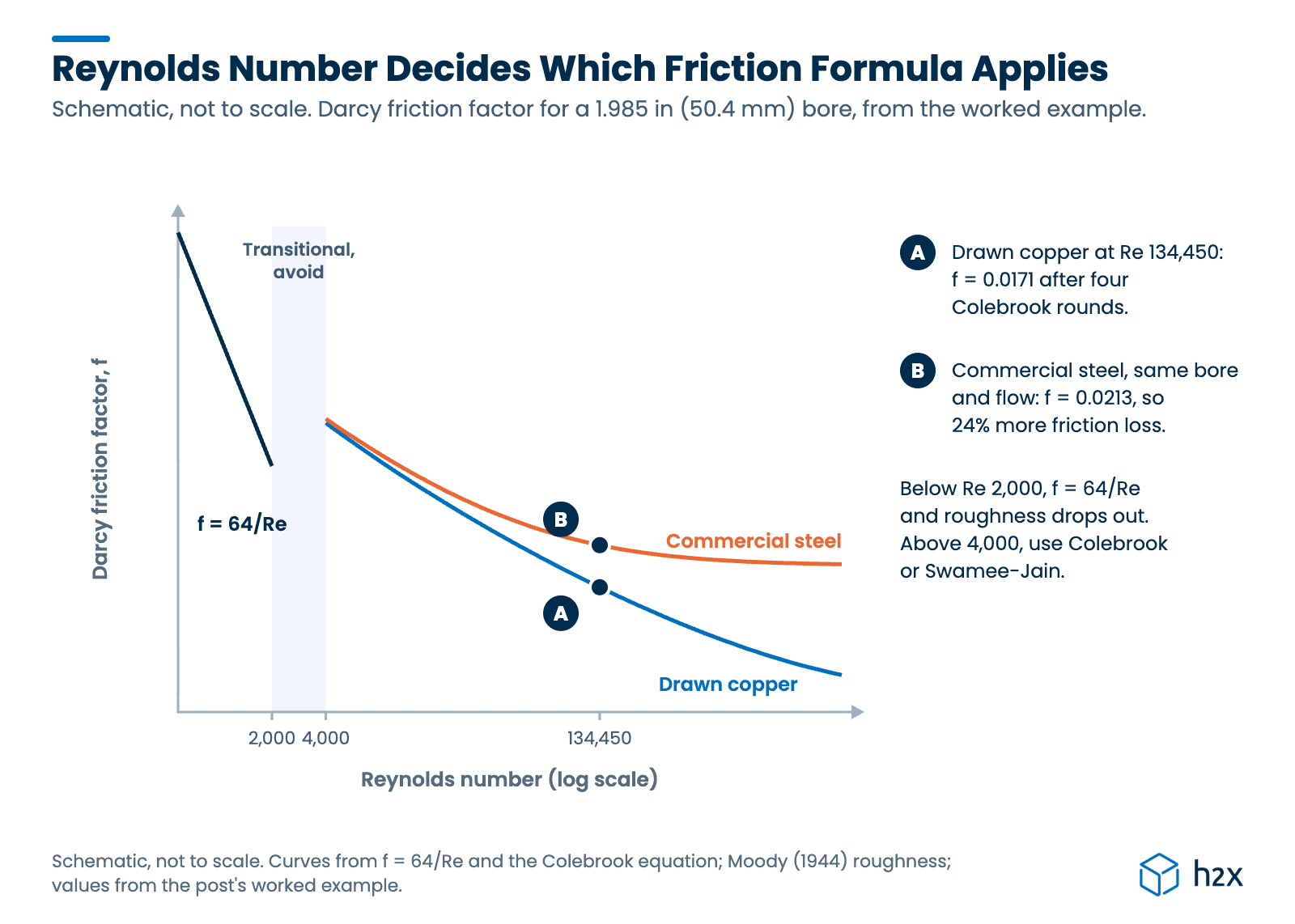
| 2,000 to 4,000 | Transitional | Unpredictable; avoid designing here |
| Above 4,000 | Turbulent | Colebrook or Swamee-Jain |
For a rectangular or other non-circular duct, swap D for the hydraulic diameter, Dh = 4A / P, where A is the cross-sectional area and P the wetted perimeter. Bentley’s hydraulic reference gives the same rule as four times the hydraulic radius.
Use Dh in the Reynolds number, in ε/D and in Darcy-Weisbach, and Colebrook then works as it does for a round pipe. In laminar flow, though, the 64 in f = 64/Re changes with the duct’s shape.
Almost every heating, chilled water and domestic water pipe runs turbulent. Laminar flow turns up in slow, viscous cases, such as a cold glycol mix at low flow.
What Is the Friction Factor Formula for Laminar Flow?
In laminar flow, the Darcy friction factor depends on the Reynolds number alone:
f = 64 / Re
Roughness drops out, because the slow layers of fluid near the wall don’t trip over it. At Re 2,000 that gives f = 0.032, the top of the laminar range.
What Is the Colebrook Equation?
The Colebrook equation gives the Darcy friction factor in turbulent flow from the Reynolds number and the relative roughness, ε/D. C. F. Colebrook published it in 1939 in the Journal of the Institution of Civil Engineers. It’s also the curve behind the Moody chart:
1 / √f = −2 log₁₀( ε / (3.7D) + 2.51 / (Re √f) )
Here ε is the absolute roughness of the pipe wall and D the internal diameter, in the same units. Because f appears on both sides, you can’t solve it in one step. Instead you guess f, put it into the right-hand side, and repeat until the answer stops changing. In practice that takes three or four rounds from a starting guess of 0.02, as the worked example below shows. The bracket holds two terms, and whichever is larger decides how much the pipe’s roughness matters.

How Do You Read a Moody Chart?
The Moody chart plots the Colebrook equation, so it’s the visual alternative to iterating. Find your Reynolds number on the bottom axis, then follow it up to the curve for your relative roughness, ε/D, marked down the right-hand side. Read the Darcy friction factor off the left-hand axis. Expect to read only two significant figures, so use the chart to check a calculated value rather than replace it.
What Is the Swamee-Jain Equation?
The Swamee-Jain equation is an explicit approximation of Colebrook, so it gives f in one step:
f = 0.25 / [ log₁₀( ε / (3.7D) + 5.74 / Re^0.9 ) ]²
P. K. Swamee and A. K. Jain published it in 1976 in the Journal of the Hydraulics Division of ASCE. Comparison studies, such as this one in Engenharia Agrícola, put it within about 1% of Colebrook across most turbulent pipe flows. In the worked example below it lands within 0.7%, which makes it a good quick check on a Colebrook result.
What Pipe Roughness Should You Use?
Absolute roughness, ε, is the average height of the bumps on the pipe wall. These values come from Moody’s 1944 paper in the Transactions of the ASME:
| Pipe material | Absolute roughness, ft (mm) |
|---|---|
| Drawn tubing (copper, brass) | 0.000005 (0.0015) |
| Commercial steel or wrought iron | 0.00015 (0.046) |
| Cast iron | 0.00085 (0.26) |
These are values for clean, new pipe. Older steel and iron pipe gets rougher as scale builds up. So check your project’s design basis for the value it expects.
Roughness Values h2x Uses
h2x stores roughness for each pipe and duct material, and for pipes it varies with the standard or manufacturer you pick. That’s why some rows below are ranges.
| Pipe material | Absolute roughness, ft (mm) |
|---|---|
| Copper | 0.000005 to 0.00001 (0.0015 to 0.003) |
| Stainless steel | 0.000005 to 0.000015 (0.0015 to 0.0046) |
| PEX | 0.000005 to 0.000023 (0.0015 to 0.007) |
| Carbon steel and seamless steel | 0.00015 (0.046) |
| Galvanized mild steel (GMS) | 0.00015 to 0.0005 (0.046 to 0.15) |
| Duct material | Absolute roughness, ft (mm) |
|---|---|
| Aluminium, carbon steel and PVC | 0.0001 (0.03) |
| Galvanized steel | 0.00025 (0.075) |
| Hot-dip galvanized steel | 0.0005 (0.15) |
| Semi-rigid duct | 0.0016 (0.5) |
| Fibrous glass duct | 0.0030 (0.9) |
| Flexible duct | 0.0098 (3.0) |
Flexible duct is about 100 times rougher than sheet steel, which is one reason long flex runs eat so much fan pressure. Our air duct pressure drop guide covers the duct side in full.
Darcy Friction Factor Worked Example
This illustrative example finds the friction factor for a copper heating hot water main. Then it repeats the sums for steel of the same bore. The water properties are NIST’s figures for 140 °F (60 °C), and the bore comes from the Copper Development Association’s Type L table.
| Input | US | Metric |
|---|---|---|
| Pipe | Type L copper, 2 in trade size, 1.985 in internal diameter | 50.4 mm internal diameter |
| Flow | 40 gpm | 2.52 L/s |
| Water temperature | 140 °F | 60 °C |
| Density | 61.38 lb/ft³ | 983.2 kg/m³ |
| Dynamic viscosity | 3.13 × 10⁻⁴ lb/(ft·s) | 0.466 mPa·s |
| Roughness, drawn copper | 0.000005 ft | 0.0015 mm |
Step 1. Velocity and Reynolds Number
First, the bore area is 0.0215 ft² (19.97 cm²), so the velocity is 4.15 ft/s (1.26 m/s). With the density and viscosity above, Re = ρVD / μ comes to 134,450. That’s well above 4,000, so the flow is turbulent and Colebrook applies.
Step 2. Relative Roughness
Relative roughness is the roughness divided by the bore. Here that’s 0.000005 ft (0.0015 mm) over a 0.1654 ft (50.4 mm) bore, so ε/D = 0.000030. At the final answer, the roughness term inside the Colebrook bracket, ε/(3.7D), is just 0.0000082, against 0.000143 for the Reynolds term. So drawn copper is smooth enough that the Reynolds term, more than 17 times larger, sets the result.
Step 3. Solve Colebrook
Starting from f = 0.02, each round feeds the last answer back into the equation:
| Round | f |
|---|---|
| Start | 0.02000 |
| 1 | 0.01684 |
| 2 | 0.01715 |
| 3 | 0.01712 |
| 4 | 0.01712 |
So the Darcy friction factor is 0.0171 after four rounds. For comparison, Swamee-Jain gives 0.0170 in one step, 0.6% lower. The Fanning value would be 0.00428.
Step 4. Friction Loss
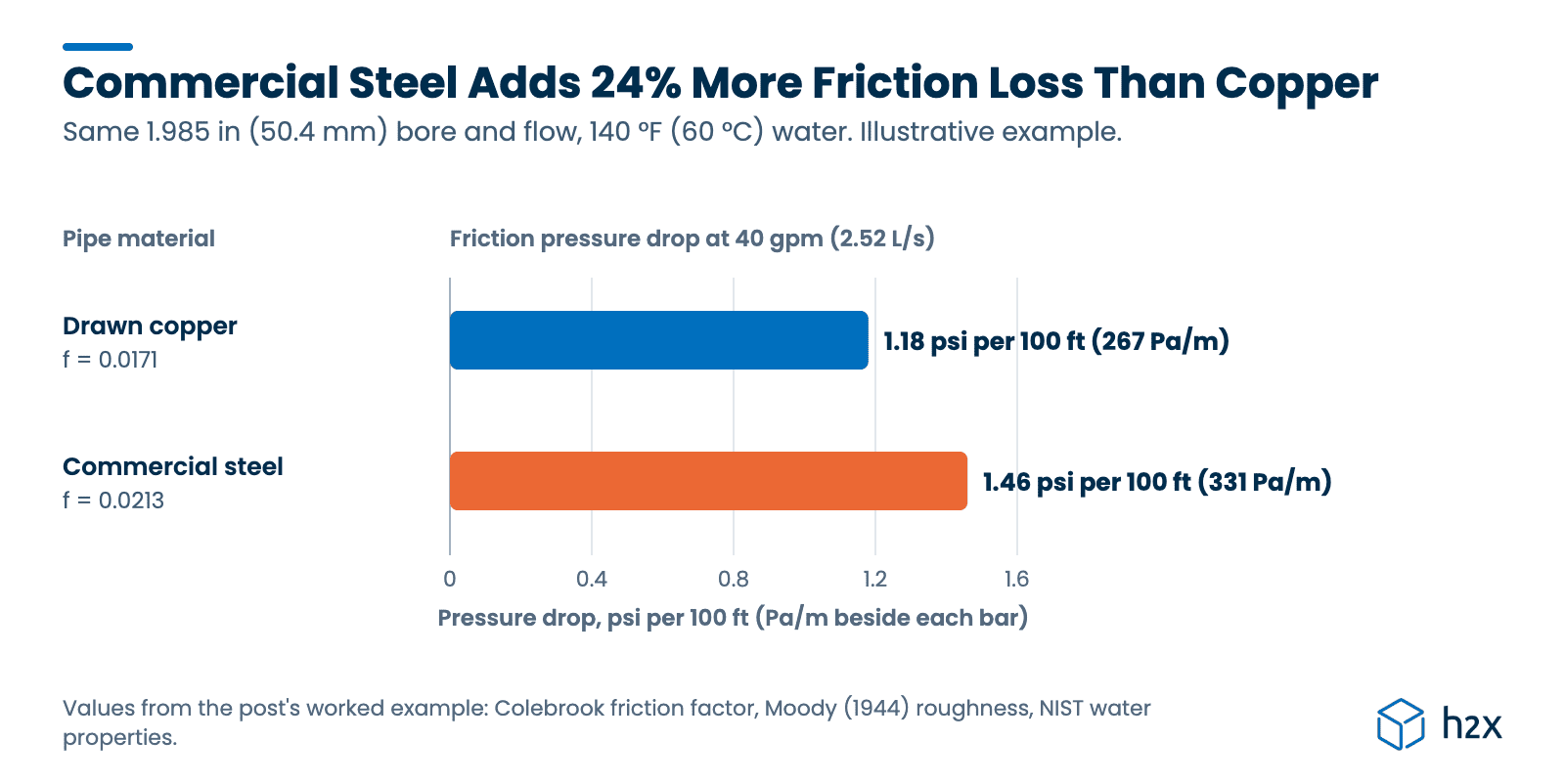
Putting f into Darcy-Weisbach gives a friction loss of 2.77 ft per 100 ft (2.77 m per 100 m). As pressure, that’s 1.18 psi per 100 ft (267 Pa/m).
Step 5. The Same Bore in Commercial Steel
Swap the roughness for commercial steel, 0.00015 ft (0.046 mm), and ε/D rises to 0.000907. Colebrook now settles at f = 0.0213 in three rounds, and Swamee-Jain gives 0.0214. Inside the bracket, the roughness term is now 0.000245, nearly twice the Reynolds term of 0.000128, so roughness has taken over.
The friction loss climbs to 3.44 ft per 100 ft (3.44 m per 100 m), or 1.46 psi per 100 ft (331 Pa/m). That’s 24% more than copper for the same flow.
Typical Darcy Friction Factor Values
These values come from the Colebrook equation for the same 1.985 in (50.4 mm) bore. They’re a sanity check, not a substitute for running your own numbers.
| Reynolds number | Drawn copper | Commercial steel |
|---|---|---|
| 2,000 (laminar, either pipe) | 0.032 | 0.032 |
| 10,000 | 0.0309 | 0.0322 |
| 100,000 | 0.0182 | 0.0219 |
| 1,000,000 | 0.0123 | 0.0195 |
So most turbulent building services pipework sits between about 0.012 and 0.032. If yours falls well outside that, check the Reynolds number, the roughness units and whether a formula wants Fanning.
Common Mistakes
- Reading a Fanning chart as Darcy. A Fanning value is a quarter of the Darcy value, so dropping one into Darcy-Weisbach understates the loss fourfold.
- Using the nominal diameter. Type L copper in the 2 in trade size has a 1.985 in (50.4 mm) bore. Use the internal diameter for Re and ε/D.
- Using roughness for new pipe on old steel. Scale makes steel and iron rougher with age. Check the value your design basis calls for.
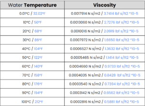
- Taking water properties at the wrong temperature. Viscosity falls as water heats, which raises Re and lowers f. So look up properties at the design temperature. Our glycol guide covers mixtures.
- Designing in the transitional band. Between Re 2,000 and 4,000 the friction factor jumps around. So pick a pipe size that keeps you clear.
How h2x Helps with the Darcy Friction Factor
Charts and tables are fine for a sanity check, but they assume a water temperature and a roughness that rarely match your job. So h2x engineering software uses CIBSE-verified calculations instead: Darcy-Weisbach with the Colebrook-White friction factor, solved for every pipe at your own design conditions.
As you draw, h2x takes care of the rest:
- Re and f for every pipe, from the material you pick and the design temperature you enter.
- A full recalculation when you resize a pipe from 1¼ in to 1½ in (32 mm to 40 mm), so velocity, f and pressure drop stay current across the system.
- Roughness from the pipe database, so there’s no hunting through tables.
- Drawings, calculations and a bill of materials ready to export to Revit, AutoCAD and PDF as the layout changes.
For a quick standalone check, try our pressure drop calculator or the pipe velocity calculator.
Key Takeaways
The Darcy friction factor turns pipe roughness and flow conditions into the single number Darcy-Weisbach needs. Find the regime from the Reynolds number first, then use f = 64/Re for laminar flow and Colebrook for turbulent flow.
- Laminar flow: below Re 2,000, the Darcy friction factor is
f = 64 / Reand roughness doesn’t matter. - Turbulent flow: above Re 4,000, solve the Colebrook equation by iteration, which usually converges in three or four rounds.
- Swamee-Jain: the explicit shortcut stayed within 0.7% of Colebrook in this guide’s worked example.
- Worked example: 40 gpm (2.52 L/s) of 140 °F (60 °C) water in a 1.985 in (50.4 mm) copper bore gives f = 0.0171.
- Roughness: the same bore in commercial steel gives f = 0.0213 and 24% more friction loss.
- h2x: h2x works out f for every pipe from the design temperature you enter, then applies Darcy-Weisbach.
FAQ
What is a typical Darcy friction factor?
For turbulent flow in clean building services pipework, the Darcy friction factor is usually between about 0.012 and 0.032. Smooth copper sits at the low end, around 0.018 at Re 100,000. But commercial steel of the same bore is nearer 0.022. And laminar flow at Re 2,000 gives 0.032.
What is the difference between the Darcy friction factor and the Fanning factor?
Both describe the same wall friction, but the Darcy factor is defined to be four times the Fanning factor. Fanning shows up mostly in chemical engineering texts, while building services references and Darcy-Weisbach use Darcy. So a Fanning value dropped into Darcy-Weisbach gives a friction loss a quarter of the true figure.
Is the Colebrook or Swamee-Jain equation more accurate?
The Colebrook equation is the reference, because Swamee-Jain was fitted to it. Swamee-Jain avoids the iteration and usually lands within about 1% of Colebrook. In this guide’s worked example it was within 0.7%. So use Colebrook for final sizing and Swamee-Jain for quick checks and spreadsheets.
Does the Darcy friction factor have units?
No. The Darcy friction factor is dimensionless, so it’s the same number in US and SI units. What matters is consistent units inside the Reynolds number and the relative roughness. For example, put roughness and diameter both in ft or both in mm.
Size Chilled Water Pipes at Their Real Viscosity
h2x applies Darcy-Weisbach to chilled water pipework at the design temperature you enter. Change that temperature and every friction factor and pressure drop updates with it.
Meet the author

Daniel Mousdell
Daniel Mousdell is the Founding Marketer at h2x, where he creates technical content and resources for HVAC and MEP engineers. Outside of work, he runs LilWayneHQ.
Article published: February 3, 2026
Last updated: October 13, 2026
Technically reviewed by: Jonathan Mousdell, Mechanical Engineer and Co-founder at h2x